mars_cnn
Mars Image Classification
by Alex Neal (alexneal.net) on September 8, 2020
In Deep Mars: CNN Classification of Mars Imagery for the PDS Imaging Atlas [1], Wagstaff et al. introduced the HiRise Orbital Dataset for the purpose of training a CNN to categorize Martian landmarks, such as craters and dunes. The dataset consists of 3820 grayscale JPEG images of the Mars surface. Each 227x227 pixel image is cropped from one of 168 larger images taken by a high resolution camera onboard the Mars Reconnaisance Orbiter.
The authors’ published model is a fine-tuned version of the well-known AlexNet CNN [2], which was initially trained on 1.2 million images belonging to 1000 different classes. This method of leveraging additional data, known as transfer learning, has proven effective in computer vision applications.
For this experiment, we will attempt to maximize the performance of a CNN trained from scratch, and compare this performance to Wagstaff et al’s transfer learning approach. We will tune hyperparameters by defining a hyperparameter space and performing a random search. The most effective set of hyperparameters from the search will be used in our final model.
We begin by importing the modules we will be using. These include:
- Tensorflow and Keras for building and training the CNN
- Keras Tuner for optimizing hyperparameters
- NumPy
- matplotlib.pyplot for visualizations
- Some other helpful utilities
from tensorflow import keras
from tensorflow.keras import layers
from kerastuner.tuners import RandomSearch
import numpy as np
import matplotlib.pyplot as plt

from PIL import Image
from tqdm import tqdm
from sklearn.model_selection import train_test_split
from sklearn.metrics import confusion_matrix, ConfusionMatrixDisplay
import IPython
Data Import and Preprocessing
The dataset includes two files and a folder of images. The first file, landmarks_mp.py, contains a dictionary for mapping the numeric class labels to the class names. We’ll add this to the execution environment for later use.
class_map = {0: 'other',
             1: 'crater',
             2: 'dark_dune',
             3: 'streak',
             4: 'bright_dune',
             5: 'impact',
             6: 'edge'}
The second file, labels-map-proj.txt, contains space-separated image filenames and correspondong class labels. The first task is to partition these lines randomly into training, validation, and test sets. We use the same proportions as the original authors: 70%, 15%, and 15% for the training, validation, and test sets, respectively.
file = open('labels-map-proj.txt', 'r')
lines = [line.strip() for line in file.readlines()]
file.close()

train, not_train = train_test_split(lines, train_size=0.7)
val, test = train_test_split(not_train, test_size=0.5)
Next, we import the image data and store them and the labels in NumPy arrays.
img_path = 'map-proj/'

def get_set(lines):
  images = []
  labels = []

  for line in tqdm(lines):
    filename, label = line.split(' ')
    images.append(np.array(Image.open(img_path + filename)
    labels.append(int(label))

  images = np.array(images)
  labels = np.array(labels)

  return images, labels


print("Importing training set...")
train_images, train_labels = get_set(train)

print()
print("Importing validation set...")
val_images, val_labels = get_set(val)

print()
print("Importing test set...")
test_images, test_labels = get_set(test)
Output:
Importing training set...
100%|██████████| 2674/2674 [00:02<00:00,  922.92it/s]

Importing validation set...
100%|██████████| 573/573 [00:00<00:00,  945.97it/s]

Importing test set...
100%|██████████| 573/573 [00:00<00:00,  936.94it/s]
Let’s have a look at the range of pixel values in the image data.
print(train_images.min(), train_images.max())
Output:
0 255
This is the standard scaling for pixel intensity in JPEG images. Before feeding them to the network, we want to normalize these values to be in the range [0,1].
train_images = train_images/255.0
val_images = val_images/255.0
test_images = test_images/255.0
Using the image data and the previously defined class map, we can display some of the images along with the classes they belong to.
plt.figure(figsize=(10,10))
for i in range(15):
    plt.subplot(5,5,i+1)
    plt.xticks([])
    plt.yticks([])
    plt.grid(False)
    plt.imshow(train_images[i], cmap=plt.cm.binary_r)
    plt.xlabel(class_map[train_labels[i]])
plt.show()
Output:
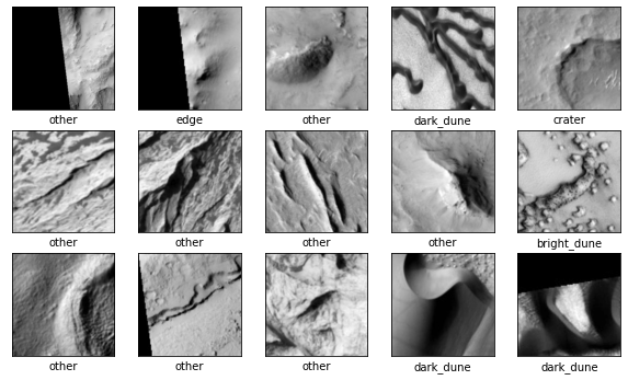
It looks like the “other” category may be more common than the others. Let’s take a look at the normalized distribution of the labels in each set.
def plot_class_dist(labels, title):
  classes, counts = np.unique(labels, return_counts=True)
  classes = [class_map[label] for label in classes]
  normalized_counts = (counts/counts.sum())
  plt.bar(classes, normalized_counts)
  plt.title(title)
  plt.xticks(rotation=90)


plt.figure(figsize=(10,2))
plt.subplot(1,3,1)
plot_class_dist(train_labels, 'Training')
plt.subplot(1,3,2)
plot_class_dist(val_labels, 'Validation')
plt.subplot(1,3,3)
plot_class_dist(test_labels, 'Testing')
plt.show()
Output:
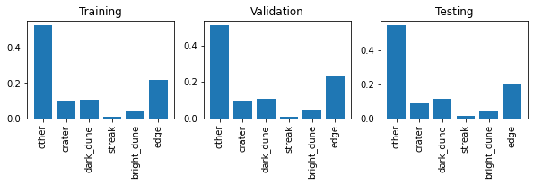
Indeed, the majority of images fall into the “other” class, which is the label for landmarks that do not fit into any of the more explicit classes. The relative class proportions in the validation and testing sets look about the same as those in the training set. This indicates that the validation and testing sets are sufficiently large, i.e. they are each acceptable representative samples of the whole dataset.
Before we can start tuning and training, there is one last step. If we look at the shape of the image data, we see that each example is a 227x227 array.
print(train_images.shape, val_images.shape, test_images.shape)
Output:
(2674, 227, 227) (573, 227, 227) (573, 227, 227)
The Keras Conv2D layer expects each training example to be a 3D tensor in which the first two dimensions are the length and width of the image, and the third dimension is the number of channels. Since these are grayscale images, they only have a single channel. We can simply reshape the arrays to add this dimension.
train_images = train_images.reshape((train_images.shape[0],227,227,1))
val_images = val_images.reshape((val_images.shape[0],227,227,1))
test_images = test_images.reshape((test_images.shape[0],227,227,1))

print(train_images.shape, val_images.shape, test_images.shape)
Output:
(2674, 227, 227, 1) (573, 227, 227, 1) (573, 227, 227, 1)
Define a Hyperparameter Space and a Model Building Function
The first step in using keras tuner is to define a hyperparameter space that can be searched. We’ll use some of the established wisdom on CNN architecture, including the architecture of AlexNet, to inform the space definition.
The first layer will be a convolutional layer with either 32, 64, 96, or 128 filters. The filter size for this layer will be either 3x3, 5x5, or 11x11, and the stride will be either 1 or 2. We will also allow for an even larger stride of 4 in cases where the 11x11 filter is chosen (The first layer of AlexNet consists of 11x11 filters with a stride of 4, so I wanted to make sure this combination was included in the search space). This layer is followed by a 2x2 max pool.
The aforementioned layer will be followed by between one and four additional convolutional layers. These layers can also have either 32, 64, 96, or 128 filters. Filter size can be 3x3 or 5x5, and the stride will be 1. Only the final layer from this group will be followed by a max pool.
There may be anywhere between one and four fully connected layers after the last max pool, and each of these layers can have a minimum of 64 and a maximum of 512 neurons. Additionally, each fully connected layer is optionally followed by a 50% dropout layer.
The final layer in the model is a 7 unit softmax layer which will output the predicted probabilities for each class.
We will also add two learning rates (0.001 and 0.0001) and two optimizer choices (Adam and RMSProp) to the hyperparameter space. These learning rates and optimizers have proven effective on this problem during initial experiments.
The following code block is a model building function that defines the above hyperparameter space for the keras tuner.
def build_model(hp):
    model = keras.Sequential()

    # convolutional / max pooling layers
    # For first layer, only make large stride of 4 possible if filter size is 11x11
    layer_1_filtersize = hp.Choice('filtersize_1', values=[3,5,11])
    if layer_1_filtersize == 11:
      possible_strides = [1,2,4]
    else:
      possible_strides = [1,2]
    model.add(layers.Conv2D(hp.Choice('filters_1', values=[32,64,96,128]),
                            layer_1_filtersize,
                            strides=hp.Choice('strides_1', values=possible_strides),
                            activation='relu',
                            input_shape=train_images.shape[1:]))

    model.add(layers.MaxPooling2D((2,2)))

    # Up to 4 additional conv layers
    for i in range(hp.Int('num_conv_layers', 1, 4)):
      model.add(layers.Conv2D(hp.Choice('filters_' + str(i+2), values=[32,64,96,128]),
                              hp.Choice('filtersize_' + str(i+2), values=[3,5]),
                              activation='relu'))

    model.add(layers.MaxPooling2D((2,2)))
    model.add(layers.Flatten())


    # fully connected layers (up to four)
    for i in range(hp.Int('num_dense_layers', 1, 4)):
      model.add(layers.Dense(units=hp.Int('dense_units_' + str(i+1),
                                          min_value=64,
                                          max_value=512,
                                          step=64),
                                          activation='relu'))
      if hp.Choice('dropout_dense_' + str(i+1), values=[True,False], default=False):
        model.add(layers.Dropout(0.5))

    # output softmax layer
    model.add(layers.Dense(7, activation='softmax'))

    # learning rate & optimizer
    learning_rate = hp.Choice('learning_rate', values=[0.001, 0.0001])

    if hp.Choice('optimizer', values=['adam', 'rmsprop']) == 'adam':
      model.compile(optimizer=keras.optimizers.Adam(learning_rate),
          loss='sparse_categorical_crossentropy',
          metrics=['accuracy'])
    else:
      model.compile(optimizer=keras.optimizers.RMSprop(learning_rate),
          loss='sparse_categorical_crossentropy',
          metrics=['accuracy'])

    return model
Tune Hyperparameters
Now we can use our model building function to initialize the random search tuner. We’ll instruct the tuner to select the hyperparameters that produce the highest validation accuracy during the tuning process. The tuner will try 40 different sets of hyperparameters, and repeat each trial three times for a higher degree of result reliability.
tuner = RandomSearch(
    build_model,
    objective='val_accuracy',
    max_trials=30,
    executions_per_trial=3,
    overwrite=True,
    project_name='mars_trials')

# Uncomment to view summary of search space
# tuner.search_space_summary()
keras tuner is quite verbose, so let’s also define a quick callback to clear the output after each trial:
class ClearTrainingOutput(keras.callbacks.Callback):
  def on_train_end(*args, **kwargs):
    IPython.display.clear_output(wait = True)
Finally, we begin tuning. In initial experiments, the network took between 20 and 30 epochs to minimize validation loss. We’ll allow each trial to run for 30 epochs to ensure that each model has the opportunity to converge.
tuner.search(train_images, train_labels,
             validation_data=(val_images, val_labels),
             epochs=30,
             callbacks=[ClearTrainingOutput()])
This tuning process took approximately two hours on a GPU hosted by Google Colab. After completion, we can retrieve the set of hyperparameters that achieved the highest performance:
best_hp = tuner.get_best_hyperparameters()[0]

best_model = tuner.hypermodel.build(best_hp)
best_model.summary()
Output:
Model: "sequential"
_________________________________________________________________
Layer (type)                 Output Shape              Param #
=================================================================
conv2d (Conv2D)              (None, 109, 109, 32)      3904
_________________________________________________________________
max_pooling2d (MaxPooling2D) (None, 54, 54, 32)        0
_________________________________________________________________
conv2d_1 (Conv2D)            (None, 52, 52, 32)        9248
_________________________________________________________________
conv2d_2 (Conv2D)            (None, 48, 48, 96)        76896
_________________________________________________________________
max_pooling2d_1 (MaxPooling2 (None, 24, 24, 96)        0
_________________________________________________________________
flatten (Flatten)            (None, 55296)             0
_________________________________________________________________
dense (Dense)                (None, 320)               17695040
_________________________________________________________________
dropout (Dropout)            (None, 320)               0
_________________________________________________________________
dense_1 (Dense)              (None, 320)               102720
_________________________________________________________________
dropout_1 (Dropout)          (None, 320)               0
_________________________________________________________________
dense_2 (Dense)              (None, 384)               123264
_________________________________________________________________
dense_3 (Dense)              (None, 192)               73920
_________________________________________________________________
dense_4 (Dense)              (None, 7)                 1351
=================================================================
Total params: 18,086,343
Trainable params: 18,086,343
Non-trainable params: 0
_________________________________________________________________
The summary above does not include the stride for the first convolutional layer, the filter sizes for all convolutional layers, the learning rate, or the optimizer. We can directly retrieve each of these hyperparameter selections as follows:
for i in range(best_hp.get('num_conv_layers')+1):
  filter_size = best_hp.get('filtersize_' + str(i+1))
  print('Filter Size (conv layer {}): {}x{}'.format(i+1, filter_size, filter_size))
print('Stride (conv layer 1): ', best_hp.get('strides_1'))
print('Learning Rate: ', best_hp.get('learning_rate'))
print('Optimizer: ', best_hp.get('optimizer'))
Output:
Filter Size (conv layer 1): 11x11
Filter Size (conv layer 2): 3x3
Filter Size (conv layer 3): 5x5
Stride (conv layer 1):  2
Learning Rate:  0.0001
Optimizer:  rmsprop
So, our network will use the RMSprop optimizer with an initial learning rate of 0.0001. A layer-by-layer summary of the chosen architecture is:
- Input layer accepting single channel 2D arrays of size 227x227
- Convolutional layer with 32 11x11 filters and stride of 2
- 2x2 max pooling layer
- Convolutional layer with 32 3x3 filters and stride of 1
- Convolutional layer with 96 5x5 filters and stride of 1
- 2x2 max pooling layer
- Fully connected layer with 320 neurons
- 50% dropout layer
- Fully connected layer with 320 neurons
- 50% dropout layer
- Fully connected layer with 384 neurons
- Fully connected layer with 192 neurons
- Output softmax layer with 7 units
Training
Having established the hyperparameters, we can now train our final network. To prevent overfitting, we will pass an early stopping callback to halt training after 4 epochs of no validation loss improvement.
history = best_model.fit(train_images, train_labels, epochs=30,
                validation_data=(val_images, val_labels),
                callbacks=[keras.callbacks.EarlyStopping(monitor='val_loss', patience=4)])
Output:
Epoch 1/30
84/84 [==============================] - 2s 19ms/step - loss: 1.2772 - accuracy: 0.5774 - val_loss: 0.9578 - val_accuracy: 0.7068
Epoch 2/30
84/84 [==============================] - 1s 16ms/step - loss: 0.9653 - accuracy: 0.7004 - val_loss: 0.9733 - val_accuracy: 0.7138
Epoch 3/30
84/84 [==============================] - 1s 17ms/step - loss: 0.9037 - accuracy: 0.7091 - val_loss: 0.8605 - val_accuracy: 0.7155
Epoch 4/30
84/84 [==============================] - 1s 17ms/step - loss: 0.8765 - accuracy: 0.7091 - val_loss: 0.8592 - val_accuracy: 0.7173
Epoch 5/30
84/84 [==============================] - 1s 17ms/step - loss: 0.8726 - accuracy: 0.7139 - val_loss: 0.8504 - val_accuracy: 0.7243
Epoch 6/30
84/84 [==============================] - 1s 17ms/step - loss: 0.8367 - accuracy: 0.7177 - val_loss: 0.8118 - val_accuracy: 0.7173
Epoch 7/30
84/84 [==============================] - 1s 17ms/step - loss: 0.8003 - accuracy: 0.7162 - val_loss: 0.7876 - val_accuracy: 0.7138
Epoch 8/30
84/84 [==============================] - 1s 17ms/step - loss: 0.7721 - accuracy: 0.7199 - val_loss: 0.7934 - val_accuracy: 0.7190
Epoch 9/30
84/84 [==============================] - 1s 16ms/step - loss: 0.7343 - accuracy: 0.7289 - val_loss: 0.7010 - val_accuracy: 0.7679
Epoch 10/30
84/84 [==============================] - 1s 17ms/step - loss: 0.6854 - accuracy: 0.7625 - val_loss: 0.6314 - val_accuracy: 0.7958
Epoch 11/30
84/84 [==============================] - 1s 17ms/step - loss: 0.6400 - accuracy: 0.7678 - val_loss: 0.5891 - val_accuracy: 0.7976
Epoch 12/30
84/84 [==============================] - 1s 17ms/step - loss: 0.6031 - accuracy: 0.7936 - val_loss: 0.5540 - val_accuracy: 0.8115
Epoch 13/30
84/84 [==============================] - 1s 17ms/step - loss: 0.5492 - accuracy: 0.8130 - val_loss: 0.5479 - val_accuracy: 0.8115
Epoch 14/30
84/84 [==============================] - 1s 16ms/step - loss: 0.5184 - accuracy: 0.8209 - val_loss: 0.5199 - val_accuracy: 0.8185
Epoch 15/30
84/84 [==============================] - 1s 17ms/step - loss: 0.4822 - accuracy: 0.8298 - val_loss: 0.5282 - val_accuracy: 0.8220
Epoch 16/30
84/84 [==============================] - 1s 16ms/step - loss: 0.4381 - accuracy: 0.8467 - val_loss: 0.4790 - val_accuracy: 0.8325
Epoch 17/30
84/84 [==============================] - 1s 16ms/step - loss: 0.4187 - accuracy: 0.8500 - val_loss: 0.5396 - val_accuracy: 0.8185
Epoch 18/30
84/84 [==============================] - 1s 16ms/step - loss: 0.3881 - accuracy: 0.8680 - val_loss: 0.4963 - val_accuracy: 0.8377
Epoch 19/30
84/84 [==============================] - 1s 17ms/step - loss: 0.3545 - accuracy: 0.8796 - val_loss: 0.5294 - val_accuracy: 0.8377
Epoch 20/30
84/84 [==============================] - 1s 17ms/step - loss: 0.3218 - accuracy: 0.8953 - val_loss: 0.4724 - val_accuracy: 0.8621
Epoch 21/30
84/84 [==============================] - 1s 17ms/step - loss: 0.3053 - accuracy: 0.8923 - val_loss: 0.5702 - val_accuracy: 0.8185
Epoch 22/30
84/84 [==============================] - 1s 17ms/step - loss: 0.2631 - accuracy: 0.9073 - val_loss: 0.7342 - val_accuracy: 0.8377
Epoch 23/30
84/84 [==============================] - 1s 17ms/step - loss: 0.2609 - accuracy: 0.9147 - val_loss: 0.5272 - val_accuracy: 0.8604
Epoch 24/30
84/84 [==============================] - 1s 17ms/step - loss: 0.2300 - accuracy: 0.9241 - val_loss: 0.5118 - val_accuracy: 0.8569
The early stopping function halted training after the 24th epoch. At this point, the training accuracy was 92.4%, and the validation accuracy was 85.7%.
Let’s visualize the training history. The following code, adapted from an article by Jason Brownlee [3], plots loss and accuracy as a function of epochs for both the training and validation sets.
plt.figure(figsize=(15,5))
plt.subplot(1,2,1)
plt.plot(history.history['accuracy'])
plt.plot(history.history['val_accuracy'])
plt.title('Accuracy')
plt.ylabel('accuracy')
plt.xlabel('epoch')
plt.legend(['training', 'validation'], loc='upper left')

plt.subplot(1,2,2)
plt.plot(history.history['loss'])
plt.plot(history.history['val_loss'])
plt.title('Loss')
plt.ylabel('loss')
plt.xlabel('epoch')
plt.legend(['training', 'validation'], loc='upper right')

plt.show()
Output:
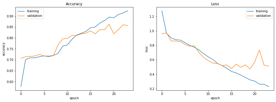
Validation accuracy and loss both seem to level out and become more volatile after the 15th epoch. Training was halted before any significant increase in validation loss, which suggests that this model is well-fit.
Evaluation
Now for the moment of truth: evaluating the model’s accuracy on the test set.
test_loss, test_accuracy = best_model.evaluate(test_images, test_labels)
print(test_accuracy)
Output:
18/18 [==============================] - 0s 8ms/step - loss: 0.6808 - accuracy: 0.8447
0.8446771502494812
The accuracy on the test set is 84.5%. Let’s have a look at the Wagstaff et al. results for comparison. The following table from the original paper includes their results along with two baselines: random-choice guessing, and always selecting the most common “other” category.
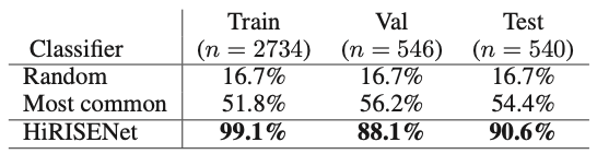
Our results of 92.4%, 85.7%, and 84.5% accuracy on our training, validation, and test sets are a bit lower than the published results of Wagstaff et al. This was to be expected since they used transfer learning and we did not. Despite that, our network is an effective predictor with accuracy that is remarkably higher than the two baselines. It is also only about 1/3 the size of the Wagstaff et al. model, with 18 million parameters compared to AlexNet’s 60 million.
Prediction
We’ll conclude by visualizing our model’s decision-making. We pass the test image data to the model’s predict function to get the predicted class probabilities for each example.
predictions = best_model.predict(test_images)
To plot the images, we need to remove the extra channel dimension we added earlier.
test_images_2d = test_images.reshape((test_images.shape[:-1]))
Using code from this TensorFlow tutorial, we visualize the first 20 predictions.
def plot_image(i, predictions_array, true_label, img):
  predictions_array, true_label, img = predictions_array, true_label[i], img[i]
  plt.grid(False)
  plt.xticks([])
  plt.yticks([])

  plt.imshow(img, cmap=plt.cm.binary_r)

  predicted_label = np.argmax(predictions_array)
  if predicted_label == true_label:
    color = 'blue'
  else:
    color = 'red'

  plt.xlabel("{} {:2.0f}% ({})".format(class_map[predicted_label],
                                100*np.max(predictions_array),
                                class_map[true_label]),
                                color=color)

def plot_value_array(i, predictions_array, true_label):
  predictions_array, true_label = predictions_array, true_label[i]
  plt.grid(False)
  plt.xticks(range(7))
  plt.yticks([])
  thisplot = plt.bar(range(7), predictions_array, color="#777777")
  plt.ylim([0, 1])
  predicted_label = np.argmax(predictions_array)

  thisplot[predicted_label].set_color('red')
  thisplot[true_label].set_color('blue')

num_rows = 10
num_cols = 2
num_images = num_rows*num_cols
plt.figure(figsize=(2*2*num_cols, 2*num_rows))
for i in range(num_images):
  plt.subplot(num_rows, 2*num_cols, 2*i+1)
  plot_image(i, predictions[i], test_labels, test_images_2d)
  plt.subplot(num_rows, 2*num_cols, 2*i+2)
  plot_value_array(i, predictions[i], test_labels)
plt.tight_layout()
plt.show()
Output:
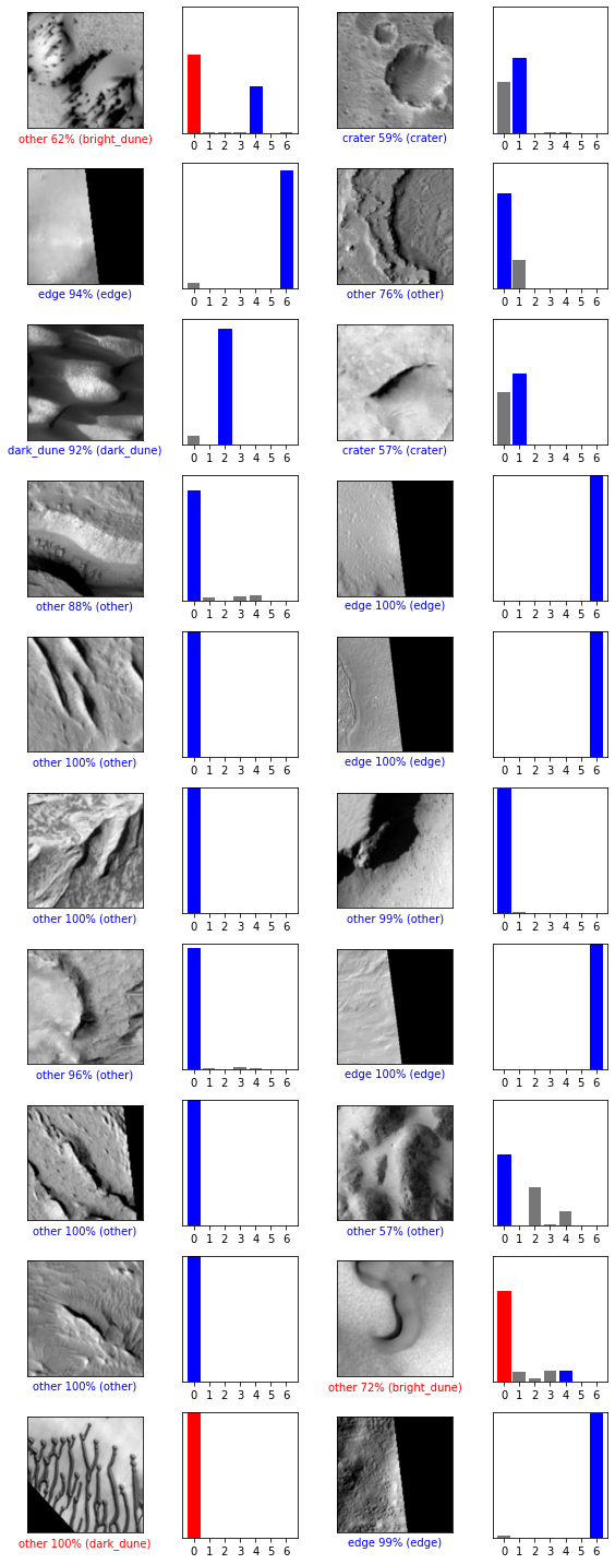
The network consistently classifies the most common categories (“other” and “edge”) correctly with a high degree of confidence. Multiple craters were also classified correctly. The network’s mistakes in this sample are all bright or dark dunes that were misclassified as “other.” The strategy, it seems, is “when in doubt, choose the most common class.”
A row-normalized confusion matrix can provide more insight into the network’s classification errors.
pred_labels = predictions.argmax(axis=1)

cm = confusion_matrix(test_labels, pred_labels, normalize='true')
display_labels = np.unique(np.concatenate((test_labels, pred_labels)))
display_labels = [class_map[label] for label in display_labels]
disp = ConfusionMatrixDisplay(confusion_matrix=cm, display_labels=display_labels)
disp = disp.plot(cmap='Blues', xticks_rotation='vertical')
plt.show()
Output:
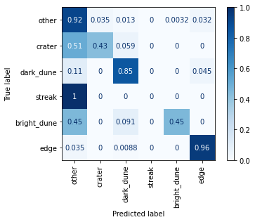
The confusion matrix shows that the model classifies images from the more common categories (“other”, “dark_dune”, and “edge”) quite effectively. There is room for significant improvement in identification of the other classes. Images in the “streak” class, for one, were classified incorrectly as “other” 100% of the time. The single best way to improve performance on these less common classes would be to increase their representation in the training set. Otherwise, transfer learning is probably the best known method for improving overall performance, as demonstrated by Wagstaff et al.
References
[1] Wagstaff, K., Y.Lu, Stanboli, A., Grimes, K., Gowda, T., & Padams, J. (2018). Deep Mars: CNN Classification of Mars Imagery for the PDS Imaging Atlas. In Conference on Innovative Applications of Artificial Intelligence.
[2] Krizhevsky, A.; Sutskever, I.; and Hinton, G. E. (2012). Imagenet Classification with Deep Convolutional Neural Networks. In Advances in Neural Information Processing Systems.
[3] Brownlee, Jason. (2016). Display Deep Learning Model Training History in Keras. At https://machinelearningmastery.com/display-deep-learning-model-training-history-in-keras/